Introduction to Linear Programs

Section 2.1 Introduction to Linear Programs

Linear programs are a special class of optimization problems in which the goal is to maximize or minimize a linear objective function subject to linear constraints. More precisely, given a linear program (LP) in \(n\) real variables \(x_1,\dots,x_n\) with \(m\) constraints is an optimization problem of the form

\begin{align*} \text{max } \amp \amp c_1x_1+c_2x_2+\cdots+c_nx_n\\ \text{subject to } \amp \amp a_{1,1}x_1+a_{1,2}x_2+\cdots+a_{1,n}x_n\leq b_1\\ \amp \amp a_{2,1}x_1+a_{2,2}x_2+\cdots+a_{2,n}x_n\leq b_2\\ \amp \amp \vdots\\ \amp \amp a_{m,1}x_1+a_{m,2}x_2+\cdots+a_{m,n}x_n\leq b_m \end{align*}

where the quantities \(c_i,a_{j,i}\) and \(b_j\) for \(1\leq i\leq n\) and \(1\leq j\leq m\) are fixed real numbers. Sometimes, linear programs will ask to minimize the objective function rather than maximize it, or will have the constraints written with \(\geq\) as opposed to \(\leq\text{.}\) Such a linear program can be seen to be equivalent to one written as above by multiplying the objective function or both sides of the constraint by \(-1\text{.}\) The value of an LP is the maximum (or minimum, depending on the LP) value of its objective function subject to the constraints. If the constraints cannot be satisfied for any choice of variables, then the value is defined to be \(-\infty\) in the case of a maximization problem or \(\infty\) in the case of a minimization problem.

There is a convenient “matrix formulation” for linear programs. Let \(A\) be the \(m\times n\) matrix whose entry on the \(i\)th row and \(j\)th column is \(a_{i,j}\text{,}\) let \(b\) be the vector of length \(m\) where the \(i\)th entry is \(b_i\text{,}\) let \(c\) be the vector of length \(n\) whose \(j\)th entry is \(c_j\) and let \(x\) be the vector of length \(n\) whose \(j\)th entry is the variable \(x_j\text{.}\) Then the above linear program can be rewritten as

\begin{align*} \text{max } \amp \amp c^Tx\\ \text{subject to } \amp \amp Ax\leq b \end{align*}

where, if \(y\) and \(z\) are vectors of the same length, then we write \(y\leq z\) to mean that the \(i\)th entry of \(y\) is at most the \(i\)th entry of \(z\) for all \(i\text{.}\)

We consider a simple explicit example of a linear program.

Example 2.1.1.

The following is an example of a linear program in variables \(x\) and \(y\text{:}\)

\begin{align*} \text{max } \amp \amp 2x-y\\ \text{subject to } \amp \amp x+3y \leq 3\\ \amp \amp x-y\leq 2\\ \amp \amp x\geq 0\\ \amp \amp y\geq 0. \end{align*}

Let us now build up some intuition about linear programs using Example 2.1.1 as a running example.

Subsection 2.1.1 Thinking Geometrically

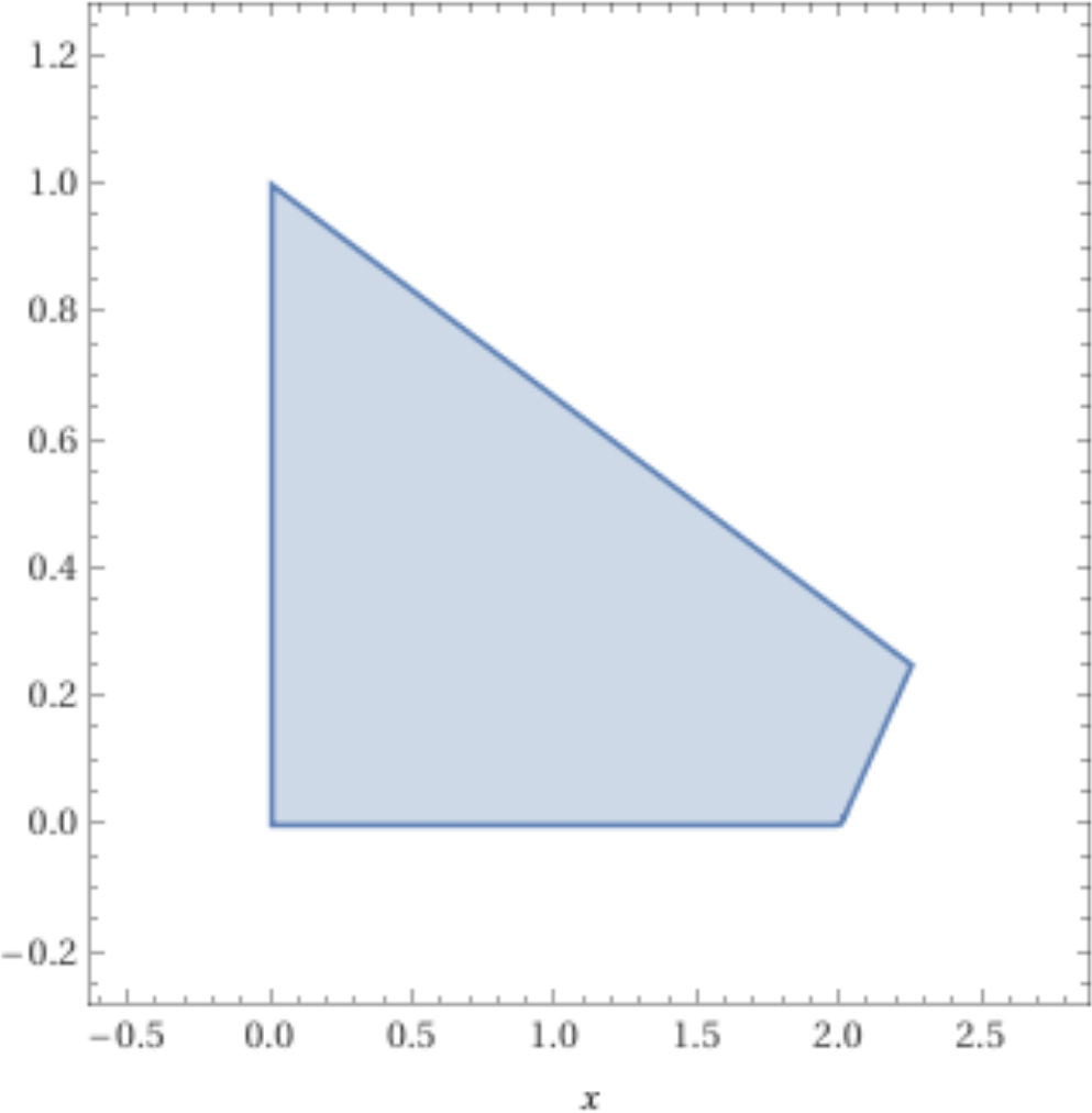
In this subsection, we will attack the optimization in Example 2.1.1 using geometric intuition and tools that you should be familiar with from Calculus. Let \(P\) be the set of all points satisfying the constraints in the linear program in Example 2.1.1; see Figure 2.1.2. Generally, we call the set \(P=\{x\in\mathbb{R}^n:Ax\leq b\}\) the feasible region for the linear program with constraints \(Ax\leq b\) and each point of the feasible region is a feasible point. If the feasible region of an LP is empty, then we call the LP infeasible and otherwise it is feasible. Coming back to our example, if we let \(f(x,y)=2x-y\text{,}\) then the standard approach from Calculus for maximizing \(f(x,y)\) on \(P\) is to

Compute the gradient of \(f\text{.}\)
Locate the critical points, i.e., the points at which the gradient is zero.
Classify the critical points using the second derivative test, or other methods.
Compute the value of \(f\) at all of the critical points on the interior of \(P\) which are candidates for being optimal (e.g. local maxima or points at which the second derivative test is inconclusive).
Find the maximum of \(f\) on the boundary of \(P\) (which may require repeating these steps for the restriction of \(f\) to the boundary).

Figure 2.1.2. The shaded area corresponds to the set \(P\) of all of the feasible points \((x,y)\) for the linear program in Example 2.1.1.

Here is where we start to notice something special about linear programs. Since our objective function is linear, the gradient is simply

\begin{equation*} \nabla f = \left(\frac{\partial f}{\partial x},\frac{\partial f}{\partial y}\right) = (2,-1). \end{equation*}

Therefore, there are no critical points, and so the maximum must be attained by a point \((x,y)\) on the boundary of \(P\text{.}\) The boundary of \(P\) consists of the following four line segments

\begin{equation*} L_1:=\{(x,y): x=0 \text{ and } 0\leq y\leq 1\}, \end{equation*}

\begin{equation*} L_2:=\{(x,y): 0\leq x\leq 9/4 \text{ and } y=1-x/3\}, \end{equation*}

\begin{equation*} L_3:=\{(x,y): x=y+2 \text{ and } 0\leq y\leq 1/4\}, \end{equation*}

\begin{equation*} L_4:=\{(x,y): 0\leq x\leq 2 \text{ and } y=0\}. \end{equation*}

The restriction of \(f\) to any of these line segments can be viewed as a linear function in only one variable. Thus, again, the maximum of \(f\) on any of these line segments is attained at the boundary of the line segment. Of course, the boundary points of these line segments are the four “corners” or “vertices” of the feasible region \(P\text{.}\) Therefore, solving the LP reduces to checking the value of \(f\) is achieved at the four vertices of the feasible region and outputting the largest value. All of the principles that we used in this specific example apply equally well to any linear program whose feasible region is bounded; there are no critical points, and so the optimum must be achieved on the boundary, and the same is true for any “face” of the feasible region, or any face of a face, and so on, until we get that the maximum is achieved at a vertex.

Recall that discrete optimization focuses on maximizing or minimizing functions over a finite domain. Prior to the observation that the maximum of an LP with bounded feasible region is achieved at a vertex, it was unclear why linear programming problems would be relevant to a course on discrete optimization. A priori, the optimum for a linear program could have been achieved at any point of the feasible region, and so the domain would seem to be infinite. However, since the optimum is achieved at a vertex, we can view such a problem as an optimization problem over a finite domain. Linear programming also carries with it the same difficulties as many discrete optimization problems. In general, the feasible region for a linear program may have a very large number of vertices relative to the size of the LP (the number of variables and constraints), and so simply computing the objective function at every vertex is often impractical and more clever methods are required to guarantee efficiency.

Now, let’s think about how we could actually solve the linear programming problem in Example 2.1.1. Since the optimum is always achieved at a vertex, we just need to determine which of the vertices is best. Imagine that we start by plotting the line \(2x-y = 0\) on top of the plot of the feasible region from Figure 2.1.2. This is a line with slope 2 through the origin and clearly intersects the set \(P\) of feasible points. Now, given a parameter \(\alpha\text{,}\) imagine plotting the line \(2x-y = \alpha\text{.}\) Every such line has slope 2 and, as \(\alpha\) increases, the line moves to the right. As long as this line intersects \(P\text{,}\) there exists a feasible point \((x,y)\) such that \(f(x,y)=\alpha\text{.}\) So, we want to push this line as far as we can to the right such that it still intersects with \(P\text{.}\) The final point at which this line will intersect \(P\) is the vertex \((x,y)=(9/4,1/4)\) yielding a maximum value of \(f(9/4,1/4)=17/4\text{.}\) Thus, the optimal value to this linear program is \(17/4\text{.}\)

Conceptually, the idea of taking the objective function \(c^Tx\) equal to a parameter \(\alpha\) and increasing it until we reach the largest \(\alpha\) such that the hyperplane \(c^Tx=\alpha\) intersects the feasible region \(\{x: Ax\leq b\}\) is a valid way of solving a linear program, but it is fairly cumbersome to turn this into an explicit algorithm and determine its running time. Also, while Example 2.1.1 involves only two variables and can therefore be visualized in the plane, a general linear program can be in any number of dimensions, making visualization impossible and requiring us to seek another method.

Instead of the “shifting hyperplane” method described in the previous paragraph, most introductory courses on linear programming introduce the Simplex Method. While the Simplex Method does not yield an efficient algorithm (nor does it have much to do with simplices), its claim to fame is that it is easy to implement and tends to perform reasonably well most of the time on linear programs that arise in real applications. We will not dwell on the details of the Simplex Method, but it is worth roughly discussing how it works in case you are not already familiar with it.

First, we start by finding a feasible point for our linear program, or showing that no feasible points exist. If the values of \(b_1,\dots,b_m\) are all non-negative, then this is easy as we can set \(x_1=x_2=\dots=x_n=0\) to get a feasible point. Otherwise, we need to first solve another LP with \(n+1\) variables \(x_1,\dots,x_n\) and \(t\) and \(m+1\) constraints described as follows

\begin{align*} \text{min } \amp \amp t\\ \text{subject to } \amp \amp a_{1,1}x_1+a_{1,2}x_2+\cdots+a_{1,n}x_n\leq b_1+t\\ \amp \amp a_{2,1}x_1+a_{2,2}x_2+\cdots+a_{2,n}x_n\leq b_2+t\\ \amp \amp \vdots\\ \amp \amp a_{m,1}x_1+a_{m,2}x_2+\cdots+a_{m,n}x_n\leq b_m+t\\ \amp \amp t\geq 0 \end{align*}

Unlike the original linear program, this one clearly has a feasible point. We can simply take \(x_1=x_2=\dots=x_n=0\) and \(t=\max_{1\leq i\leq m}|b_i|\text{.}\) So, we can apply the Simplex Method (which we will describe in a moment) to solve this linear program. If it outputs a positive optimum value for the objective function \(t\text{,}\) then we can conclude that our original LP was infeasible (can you see why?). Otherwise, the optimal point \((x_1,\dots,x_n,0)\) for the augmented linear program gives us a point that \((x_1,\dots,x_n)\) that is feasible for the original LP.

Now that we have located a feasible point \((x_1,\dots,x_n)\text{,}\) our next goal is to locate a vertex of the feasible region. To do so, start at the feasible point \((x_1,\dots,x_n)\) and move in the direction prescribed by \(c\text{,}\) which is the gradient of the objective function, until the first time that one or more of the constraints hold with equality (i.e. one of the constraints is tight). We then restrict the objective function to the affine hyperplane corresponding to points satisfying the tight inequalities and we move in the direction of its gradient of the restriction of our objective function to that hyperplane (or in an arbitrary direction if the gradient is zero) until another constraint becomes tight, and repeat this until we reach a vertex. We will know once we hit a vertex because the affine hyperplane corresponding to points satisfying the tight constraints will have dimension zero.

Now, we need to move from one vertex to another while continuing to increase the objective function. For each of the constraints that is tight at the current vertex, the set of feasible points that can be reached by relaxing that constraint only is either a line segment that starts at the current vertex and ends at another vertex or a ray that starts at the current vertex and goes to infinity. If it is the latter, and if the objective function is increasing on that ray, then the value of the LP is infinity. If this occurs, then we simply output infinity; so, from here forward, we assume that this does not happen. If there is such a line segment starting at the current vertex in which the objective function is increasing, then we choose such a line segment and follow it until we reach its other endpoint. We then repeat the process at this vertex, and keep going until we reach a vertex for which no such line segment exists. Note that we will never re-visit a vertex that we have already seen because the objective function is always strictly increasing. The final vertex that we reach via this process is the optimal point for the LP. This concludes our rough description of the Simplex Method.

While the Simplex Method does not yield an efficient method for solving linear programs in general, efficient methods do exist. The first polynomial-time algorithm for linear programming was discovered by Khachiyan in 1979 using something known as the ellipsoid method. There are now other polynomial-time algorithms, with one of the most influential being the interior-point method of Karmarkar. We will not discuss the details of these methods in this course, but will sometimes reference the important fact that linear programs can be solved in polynomial time. This is very useful because whenever we can reduce a discrete optimization problem to solving a linear program of polynomial size, then we can immediately conclude that the original problem can be solved in polynomial time.

Theorem 2.1.3. Khachiyan.

There exists an algorithm for solving linear programming problems in polynomial time with respect to the number of variables and constraints.

Subsection 2.1.2 Formalizing the Geometrical Intuition

Let us now make this geometric intuition more precise and formal. We start with the definition of a convex set.

Definition 2.1.4.

A set \(C\subseteq\mathbb{R}^n\) is said to be convex if, for all \(x,y\in C\) and \(0\leq \lambda\leq 1\text{,}\) it holds that \(\lambda x+(1-\lambda)y\in C\text{.}\)

In other words, a set \(C\) is convex if, for any two points in \(C\text{,}\) the line segment between those two points is contained in \(C\text{.}\) If you think about it intuitively and draw some pictures, you’ll see that a set is convex if it does not contain any “holes” or “indentations.” Given a set \(S\subseteq \mathbb{R}^n\text{,}\) the convex hull of \(S\) is the intersection of all convex sets \(C\) such that \(S\subseteq C\text{.}\) We write this as \(\conv(S)\text{.}\) It is not hard to see that the convex hull of a set is, itself, convex. The next lemma gives us an alternative definition of convex hull which can be more useful in practice.

Lemma 2.1.5.

For any \(S\subseteq \mathbb{R}^n\text{,}\)

\begin{equation*} \conv(S) = \left\{\sum_{i=1}^n\lambda_i x_i: n\in\mathbb{N}, x_1,\dots,x_n\in S, \lambda_1,\dots,\lambda_n\geq0, \sum_{i=1}^n\lambda_i=1\right\}. \end{equation*}

Proof.

Exercise 3.

In the previous subsection, we rambled on about “vertices” without formally defining them; let us now define this notion in the context of convex sets.

Definition 2.1.6.

Let \(C\subseteq \mathbb{R}^n\) be a convex set and \(z\in C\text{.}\) We say that \(z\) is a vertex of \(C\) if there do not exist distinct \(x,y\in C\) and \(0<\lambda<1\) such that \(z=\lambda x+(1-\lambda)y\text{.}\)

In other words, a vertex of a convex set is an “extreme point” which is not a midpoint of any line segment in \(C\text{.}\) While, in linear programming, we think of vertices as points at the “corners” of a feasible region, this is not quite the case for convex sets in general. For example, the set \(C=\{(x,y)\in \mathbb{R}^2: y\geq x^2\}\) is convex and every point \(z=(x,y)\) on the curve \(y=x^2\) is a vertex of \(C\) according to Definition 2.1.6.

A special class of convex sets that are particularly relevant in linear programming are poyhedra.

Definition 2.1.7.

A set \(P\subseteq\mathbb{R}^n\) is called a polyhedron if there exists an integer \(m\geq0\text{,}\) a real matrix \(m\times n\) matrix \(A\) and a real vector \(b\) of length \(m\) such that

\begin{equation*} P=\{x\in\mathbb{R}^n: Ax\leq b\}. \end{equation*}

A bounded polyhedron in \(\mathbb{R}^2\) is easy to visualize; it is simply a polygon. Polyhedrons can also be unbounded; for example, the entire set \(\mathbb{R}^2\) is a polyhedron, as is any closed half plane. The following video shows a bounded polyhedron in three dimensions. Generally, polyhedra are sets with “flat” faces generated by taking the intersection of finitely many half spaces (i.e. sets that lie on one side of a hyperplane).

Lemma 2.1.8.

Polyhedra are convex.

Proof.

Exercise 2.

Now, given a polyhedron \(P=\{x\in\mathbb{R}^n: Ax\leq b\}\) and a point \(z\in P\text{,}\) how can we determine whether or not \(z\) is a vertex of \(P\text{?}\) Of course, it is easy if \(P\) lives in two dimensional space (or maybe three, at a stretch) because we can plot the polyhedron and check it, but for general high dimensional linear programs, we are going to need a condition that can be checked without needing to plot it. The next definition is useful for this.

Definition 2.1.9.

Let \(P=\{x\in\mathbb{R}^n: Ax\leq b\}\) be a polyhedron where \(A\) is an \(m\times n\) matrix where the rows of \(A\) given by \(a_1,\dots,a_m\text{.}\) For \(z=(z_1,\dots,z_n)\in P\text{,}\) let \(A_z\) be the submatrix of \(A\) where a row \(a_i\) of \(A\) is included in \(A_z\) if and only if \(a_iz=b_i\text{.}\)

In other words, the matrix \(A_z\) represents all of the constraints of the LP that are tight at \(z\text{.}\) Intuitively, a point \(z\) is not a vertex of \(P\) precisely if it is possible to “wiggle both ways” around the point \(z\) in some direction while staying inside of the polyhedron \(P\text{.}\) Each of the tight constraints can be seen as restricting the possible directions in which one can move around \(z\) while staying in \(P\text{.}\) In other words, the tight constraints at \(z\) reduce the “degrees of freedom” that one can use to move around \(z\) while staying in \(P\text{.}\) For example, in Example 2.1.1, the vertices of the feasible region are precisely the points in \(P\) for which two of the constraints are tight; at each of the vertices, the matrix \(A_z\) is a \(2\times 2\) matrix and, at every other point of \(P\text{,}\) it has at most one row. From this, one might guess that the size of the matrix \(A_z\) may be the determining factor, but this is not quite right because there can be “redundancy” among the constraints. For example, if we added the constraint

\begin{equation*} 2x-2y\leq 5 \end{equation*}

to the LP in Example 2.1.1, then it would change the sizes of the matrices \(A_z\) for some points \(z\text{,}\) but it would not change the set of vertices since this inequality can be obtained by adding together the first two constraints in Example 2.1.1 and it is therefore redundant. As it turns out, the rank of the matrix \(A_z\) is the key factor which determines whether or not \(z\) is a vertices.

Lemma 2.1.10.

Let \(P=\{x\in\mathbb{R}^n: Ax\leq b\}\) be a polyhedron and let \(z\in P\text{.}\) Then \(z\) is a vertex of \(P\) if and only if the rank of \(A_z\) is \(n\text{.}\)

Proof.

Let \(a_1,\dots,a_m\) be the rows of \(A\text{.}\) First, we suppose that the rank of \(A_z\) is less than \(n\) and prove that \(z\) is not a vertex of \(P\text{.}\) Then, by the Rank–Nullity Theorem, there exists a non-zero vector \(w\) such that \(A_z w = 0\text{.}\) For any index \(i\) such that \(a_iz<b_i\text{,}\) by continuity, we can let \(\varepsilon_i>0\) so that \(a_i(z+\alpha w)<b_i\) and \(a_i(z-\alpha w)<b_i\) for all \(0<\alpha\leq \varepsilon_i\text{.}\) Let \(\varepsilon\) be the minimum of \(\varepsilon_i\) over all such indices \(i\text{.}\) Define \(x=z+\varepsilon w\) and \(y=z-\varepsilon w\text{.}\) Then, clearly, \(z=\frac{1}{2}x + \frac{1}{2}y\text{.}\) So, we will be done if we can show that \(x,y\in P\text{.}\) For any index \(1\leq i\leq m\) such that \(a_i\) is included in \(A_z\text{,}\) we have

\begin{equation*} a_i x = a_i(z + \varepsilon w) = a_iz +\varepsilon a_iw = b_i \end{equation*}

by definition of \(w\text{.}\) For any \(1\leq i\leq m\) such that \(a_i\) is not included in \(A_z\text{,}\) we have \(a_i x\leq b_i\) by definition of \(\varepsilon\text{.}\) So, \(x\in P\text{,}\) and the proof that \(y\in P\) is similar. So, \(z\) is not a vertex of \(P\text{.}\)

Now, for the converse, suppose that \(z\) is an element of \(P\) but not a vertex of \(P\text{.}\) Then there exist distinct\(x,y\in P\) and \(0< \lambda < 1\) such that \(z=\lambda x+(1-\lambda)y\text{.}\) Given a row \(a_i\) of \(A_z\text{,}\) we know that \(a_ix\leq b_i\) and \(a_iy\leq b_i\) because \(x,y\in P\text{.}\) If either of these inequalities is strict, then we would get \(a_iz=\lambda a_ix+(1-\lambda)a_iy< b_i\) which would contradict the fact that \(a_i\) is a row of \(A_z\text{.}\) However, since \(a_ix=a_iy\) for every row \(a_i\) of \(A_z\text{,}\) we have that \(A_z(x-y)=0\text{.}\) Since \(x\neq y\text{,}\) this means that \(A_z\) has non-empty kernel and so it has rank less than \(n\text{.}\) This completes the proof.

Generally speaking, polyhedra are not always bounded, and they do not always have vertices. For example, the set \(\{(x,y)\in\mathbb{R}^2: x+y\geq3\}\) is a polyhedron with no vertices, as is the entire set \(\mathbb{R}^n\) itself (by considering a constraint matrix \(A\) with zero rows). As we have seen, the maximum of a linear objective function on a bounded polyhedron is always attained at one of the vertices. The case in which the polyhedron is unbounded can be different. For one, the polyhedron may contain an infinite ray along which the objective function is increasing, in which case the maximum does not exist (i.e. the value of the LP is \(\infty\)). Also, there are situations in which the objective function is bounded on the polyhedron but does not achieve its maximum at a vertex; see Exercise 13. One needs to be very careful when dealing with linear programs over unbounded polyhedra!

If you think about it, it is fairly evident that any bounded polyhedron is equal to the convex hull of its vertices. This is indeed true, as we will state (but not prove) below.

Definition 2.1.11.

A set \(P\subseteq\mathbb{R}^n\) is called a polytope if it can be expressed as the convex hull of a finite set of points.

The next theorem tells us that polytopes and bounded polyhedra are precisely the same objects.

Theorem 2.1.12.

If \(P\) is a bounded polyhedron with vertices \(z_1,\dots,z_k\text{,}\) then \(P=\conv(\{z_1,\dots,z_k\})\text{.}\) Conversely, if \(P\) is a polytope, then it is a bounded polyhedron.

Proof.

We omit this proof from these notes. If you are interested in reading it, then please see Section 2.2 of these Lecture Notes by Alexander Schrijver.

Here is a of YouTube video related to the topics of this section.

Here is a great short video on linear programming by Bachir El Khadir which may help you build your intuition.

Prev Top Next